Preparing data and choosing sampler settings

Before calling pgmm_rjmcmc(), the analyst must specify the data orientation, scaling, missing-value handling, latent-factor dimension, cluster range, and starting covariance model.

Matrix orientation

bpgmm expects a numeric matrix with variables in rows and observations in columns. Many R data sets use the opposite convention, so transpose after selecting numeric variables.

The package convention is

$X = \begin{bmatrix} x_{11} & \cdots & x_{1n} \\ \vdots & & \vdots \\ x_{p1} & \cdots & x_{pn} \end{bmatrix},$

where row $j$ is variable $j$ and column $i$ is observation $x_i$ .

library(bpgmm)
#> bpgmm 1.3.1 loaded. If you use bpgmm in published work, please cite it with citation("bpgmm").

iris_numeric <- as.matrix(iris[, 1:4])
iris_labels <- as.integer(iris$Species)

dim(iris_numeric)
#> [1] 150   4

X <- t(iris_numeric)
dim(X)
#> [1]   4 150

Rows now correspond to variables and columns correspond to observations.

rownames(X)
#> [1] "Sepal.Length" "Sepal.Width"  "Petal.Length" "Petal.Width"
X[, 1:3]
#>              [,1] [,2] [,3]
#> Sepal.Length  5.1  4.9  4.7
#> Sepal.Width   3.5  3.0  3.2
#> Petal.Length  1.4  1.4  1.3
#> Petal.Width   0.2  0.2  0.2

Check finite numeric inputs

The sampler requires finite numeric values. Handle missing values before fitting. Common choices include complete-case filtering, domain-specific imputation, or fitting the model to a subset of variables with reliable measurements.

all(is.finite(X))
#> [1] TRUE
storage.mode(X)
#> [1] "double"

Scale variables

Mixture models are sensitive to measurement scale. If variables are measured in different units, standardizing each variable is usually a sensible default. For each variable $j$ , the usual transformation is

$x_{ji}^{\mathrm{scaled}} = \frac{x_{ji} - \bar{x}_{j\cdot}}{s_j}, \qquad s_j^2 = \frac{1}{n - 1}\sum_{i=1}^n (x_{ji} - \bar{x}_{j\cdot})^2 .$

X_scaled <- t(scale(t(X)))

round(rowMeans(X_scaled), 6)
#> Sepal.Length  Sepal.Width Petal.Length  Petal.Width 
#>            0            0            0            0
round(apply(X_scaled, 1, sd), 6)
#> Sepal.Length  Sepal.Width Petal.Length  Petal.Width 
#>            1            1            1            1

The package does not scale internally because some scientific applications need the original measurement scale. Scaling should be an explicit analysis choice.

Choose `q_new`

q_new is the latent-factor dimension assigned to newly proposed clusters. It controls the dimension of the factor-analyzer part of the covariance model. In the paper’s notation,

$\Lambda_k \in \mathbb{R}^{p \times q_k}, \qquad y_{ki} \in \mathbb{R}^{q_k}.$

The package uses q_new as the $q_k$ value for a newly created component.

Useful starting points:

q_new = 1 for very small examples or when covariance structure should be simple.
q_new = 2 or 3 for moderate-dimensional data.
Larger values only when the number of variables and observations support the extra covariance flexibility.

The value should be smaller than the number of observed variables.

p <- nrow(X_scaled)
q_new <- min(2, p - 1)
q_new
#> [1] 2

Choose `m_range`

m_range is the allowed cluster-number range. A wide range gives RJMCMC more freedom, but also increases the model space. Start with a scientifically reasonable range, then assess sensitivity.

m_init <- 3
m_range <- c(1, 5)

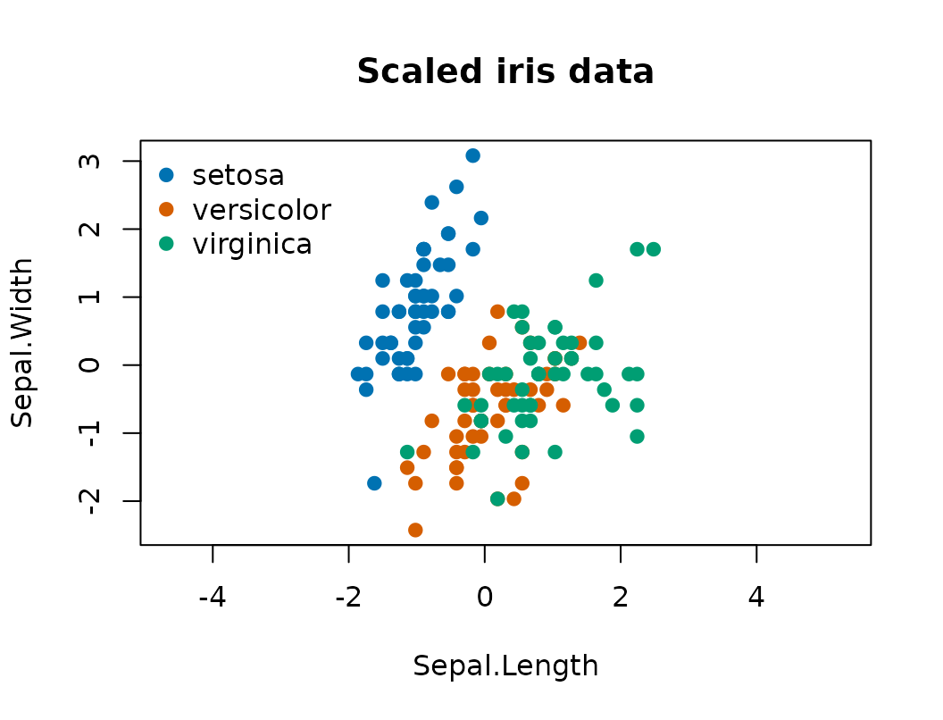
For data with a known reference label, such as iris, the reference partition gives a simple check on the range. In unsupervised applications, use domain knowledge and exploratory plots.

species_cols <- c("#0072B2", "#D55E00", "#009E73")
plot(
  X_scaled[1, ], X_scaled[2, ],
  col = species_cols[iris_labels],
  pch = 19,
  xlab = rownames(X_scaled)[1],
  ylab = rownames(X_scaled)[2],
  main = "Scaled iris data",
  asp = 1
)
legend(
  "topleft",
  legend = levels(iris$Species),
  col = species_cols,
  pch = 19,
  bty = "n"
)

Scatter plot of scaled iris variables colored by species.

Choose the starting covariance model

The three-letter model labels describe whether loading matrices and noise covariances are shared across clusters. UUU is flexible; CCC is more constrained. A flexible starting model is often reasonable when using v_step = 1, because the sampler can move across covariance structures.

The fitted covariance is always

$\Sigma_k = \Lambda_k\Lambda_k^\top + \Psi_k,$

but the label controls whether $\Lambda_k$ and $\Psi_k$ are shared and whether $\Psi_k$ is isotropic or diagonal.

model_to_constraint("UUU")
#> [1] 0 0 0
constraint_to_model(c(1, 1, 1))
#> [1] "CCC"

A prepared call

The call below is not evaluated in the vignette because applied analyses should use longer chains and repeated runs. It records how the prepared objects enter the package interface.

fit <- pgmm_rjmcmc(
  X = X_scaled,
  m_init = m_init,
  m_range = m_range,
  q_new = q_new,
  burn = 1000,
  niter = 5000,
  constraint = "UUU",
  m_step = 1,
  v_step = 1,
  split_combine = 1,
  verbose = FALSE
)

summarize_pgmm_rjmcmc(fit, true_cluster = iris_labels)

Practical checklist

Before fitting:

verify that X is numeric with variables in rows;
remove or impute missing and non-finite values;
decide whether variables should be scaled;
choose a scientifically plausible m_range;
choose q_new smaller than the number of variables;
use multiple chains for applied analyses.