Worked examples

This example gives a complete, runnable bpgmm analysis. It is small enough to build quickly on CRAN and pkgdown, but it uses the same functions as a larger analysis. The focus is the structure of one fitted object; model-selection interpretation is handled separately.

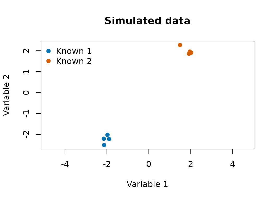
Simulate a small clustering problem

pgmm_rjmcmc() expects a numeric matrix with variables in rows and observations in columns. The code below creates two well-separated clusters in two dimensions.

library(bpgmm)
#> bpgmm 1.3.1 loaded. If you use bpgmm in published work, please cite it with citation("bpgmm").

set.seed(2026)

X <- cbind(
  matrix(rnorm(8, mean = -2, sd = 0.2), nrow = 2),
  matrix(rnorm(8, mean = 2, sd = 0.2), nrow = 2)
)
known_labels <- rep(1:2, each = 4)

dim(X)
#> [1] 2 8
known_labels
#> [1] 1 1 1 1 2 2 2 2

cluster_cols <- c("#0072B2", "#D55E00", "#009E73")
plot(
  X[1, ], X[2, ],
  col = cluster_cols[known_labels],
  pch = 19,
  xlab = "Variable 1",
  ylab = "Variable 2",
  main = "Simulated data",
  asp = 1
)
legend(
  "topleft",
  legend = paste("Known", sort(unique(known_labels))),
  col = cluster_cols[sort(unique(known_labels))],
  pch = 19,
  bty = "n"
)

Fit a fixed-model chain

This fit keeps $m$ and the covariance model fixed, so the output structure is explicit. The fitted likelihood contribution is

$$p(x_i \mid z_i = k, \Theta) = N_p(x_i \mid \mu_k, \Lambda_k\Lambda_k^\top + \Psi_k).$$

For model selection across $m$ and covariance labels, use the separate model-selection vignette.

fit_log <- capture.output({
  fit <- pgmm_rjmcmc(
    X = X,
    m_init = 2,
    m_range = c(1, 3),
    q_new = 1,
    burn = 1,
    niter = 3,
    constraint = "UUU",
    m_step = 0,
    v_step = 0,
    verbose = FALSE
  )
})
tail(fit_log, 1)
#> character(0)

The returned object stores posterior samples for allocations, covariance constraints, component parameters, and hyperparameters.

names(fit)
#>  [1] "tau_samples"            "psi_samples"           
#>  [3] "mean_samples"           "lambda_samples"        
#>  [5] "factor_score_samples"   "allocation_samples"    
#>  [7] "constraint_samples"     "alpha1_samples"        
#>  [9] "alpha2_samples"         "beta_samples"          
#> [11] "active_cluster_samples"
length(fit$allocation_samples)
#> [1] 3

Summarize posterior samples

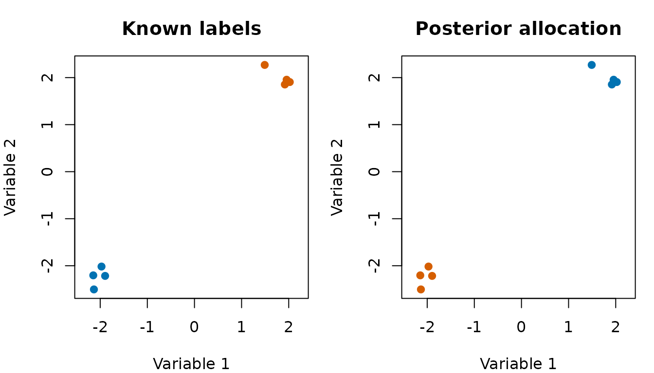
summarize_pgmm_rjmcmc() returns the modal allocation, posterior counts for the number of clusters, posterior counts for covariance models, and optionally an adjusted Rand index.

fit_summary <- summarize_pgmm_rjmcmc(fit, true_cluster = known_labels)

fit_summary$allocation
#> [1] 2 2 2 2 1 1 1 1
fit_summary$n_clusters
#> 
#> 2 
#> 3
fit_summary$n_constraints
#> 
#> UUU 
#>   3
fit_summary$ari
#> [1] 1

The modal allocation is computed coordinate-wise from the saved posterior allocations:

$$\hat{z}_i = \operatorname{mode}\{z_i^{(1)},\ldots,z_i^{(S)}\},$$

where $S$ is the number of saved posterior samples.

old_par <- par(mfrow = c(1, 2), mar = c(4, 4, 3, 1))
plot(
  X[1, ], X[2, ],
  col = cluster_cols[known_labels],
  pch = 19,
  xlab = "Variable 1",
  ylab = "Variable 2",
  main = "Known labels",
  asp = 1
)
plot(
  X[1, ], X[2, ],
  col = cluster_cols[fit_summary$allocation],
  pch = 19,
  xlab = "Variable 1",
  ylab = "Variable 2",
  main = "Posterior allocation",
  asp = 1
)

par(old_par)

Inspect component parameters

The sampler stores draws of $\tau_k$, $\mu_k$, $\Lambda_k$, and $\Psi_k$. For this fixed-model example, the final saved draw is enough to show the object shape.

last <- length(fit$tau_samples)

fit$tau_samples[[last]]
#> [1] 0.1844265 0.8155735 0.0000000
fit$mean_samples[[last]]
#> [[1]]
#>          [,1]     [,2]
#> [1,] 1.285546 1.767347
#> 
#> [[2]]
#>           [,1]      [,2]
#> [1,] -2.023394 -2.231323
#> 
#> [[3]]
#> [1] NA
lapply(fit$lambda_samples[[last]], dim)
#> [[1]]
#> [1] 2 1
#> 
#> [[2]]
#> [1] 2 1
#> 
#> [[3]]
#> NULL
lapply(fit$psi_samples[[last]], dim)
#> [[1]]
#> [1] 2 2
#> 
#> [[2]]
#> [1] 2 2
#> 
#> [[3]]
#> NULL

Scale the example to real data

For an applied analysis, keep the same sequence of steps but use larger sampler settings. The exact values depend on data size and convergence diagnostics.

fit <- pgmm_rjmcmc(
  X = your_data_matrix,
  m_init = 2,
  m_range = c(1, 10),
  q_new = 4,
  burn = 5000,
  niter = 15000,
  constraint = model_to_constraint("UUU"),
  m_step = 1,
  v_step = 1,
  split_combine = 1,
  verbose = FALSE
)

summarize_pgmm_rjmcmc(fit, true_cluster = known_labels)

What to report

For a concise analysis report, include:

• the data orientation and preprocessing choices;
• m_range, q_new, starting covariance model, and whether m_step, v_step, and split_combine were enabled;
• the number of burn-in and posterior iterations;
• the posterior modal allocation or a co-clustering matrix;
• ARI only when a reference partition is scientifically meaningful.

The diagnostics vignette gives examples of trace plots and co-clustering summaries for multiple chains.