Exploratory variable prioritization after bpgmm clustering • bpgmm

bpgmm performs Bayesian model selection for the number of clusters and PGMM covariance structure. It does not currently implement a formal spike-and-slab or inclusion-indicator variable-selection prior. Still, users often want to understand which observed variables help explain the fitted clustering.

The calculations below:

fit bpgmm;
summarize the posterior modal allocation;
rank variables by between-cluster separation;
compare that ranking with posterior loading magnitudes.

These summaries are diagnostic and exploratory. Treat them as variable prioritization, not as formal posterior variable inclusion probabilities.

Simulate data with informative and weak variables

The simulation differs from the model-selection example. The aim is not to recover $m$ , but to examine how posterior output can be post-processed to rank variables. The first three variables have different cluster means, variables four and five have mostly covariance differences, and variable six is weak noise.

library(bpgmm)
#> bpgmm 1.3.1 loaded. If you use bpgmm in published work, please cite it with citation("bpgmm").

simulate_screening_data <- function(n_per_cluster = 18, p = 6) {
  means <- rbind(
    c(-2.5, -1.5,  0.0, 0, 0, 0),
    c( 2.0, -0.5,  1.8, 0, 0, 0),
    c( 0.0,  2.2, -1.8, 0, 0, 0)
  )

  covariances <- list(
    diag(c(0.35, 0.35, 0.35, 1.40, 0.35, 1.20)),
    diag(c(0.35, 0.35, 0.35, 0.35, 1.40, 1.20)),
    matrix(c(
      0.35, 0,    0,    0,    0,    0,
      0,    0.35, 0,    0,    0,    0,
      0,    0,    0.35, 0,    0,    0,
      0,    0,    0,    1.00, 0.45, 0,
      0,    0,    0,    0.45, 1.00, 0,
      0,    0,    0,    0,    0,    1.20
    ), nrow = p)
  )

  n <- n_per_cluster * 3
  X <- matrix(NA_real_, nrow = p, ncol = n)
  true_cluster <- rep(seq_len(3), each = n_per_cluster)

  column <- 1
  for (k in seq_len(3)) {
    for (i in seq_len(n_per_cluster)) {
      X[, column] <- MASS::mvrnorm(1, mu = means[k, ], Sigma = covariances[[k]])
      column <- column + 1
    }
  }

  rownames(X) <- paste0("variable_", seq_len(p))
  list(X = X, true_cluster = true_cluster)
}

set.seed(2028)
sim <- simulate_screening_data()
X <- sim$X
true_cluster <- sim$true_cluster

The fitted PGMM still uses

$\Sigma_k = \Lambda_k\Lambda_k^\top + \Psi_k,$

but this simulation deliberately separates mean-driven variables from covariance-driven variables so the two rankings below answer different questions.

Fit a short clustering chain

fit_log <- capture.output({
  fit <- pgmm_rjmcmc(
    X = X,
    m_init = 3,
    m_range = c(1, 5),
    q_new = 2,
    burn = 2,
    niter = 6,
    constraint = "UUU",
    m_step = 1,
    v_step = 1,
    verbose = FALSE
  )
})
tail(fit_log, 1)
#> character(0)

fit_summary <- summarize_pgmm_rjmcmc(fit, true_cluster = true_cluster)
fit_summary$ari
#> [1] 0.5278689

Rank variables by posterior allocation separation

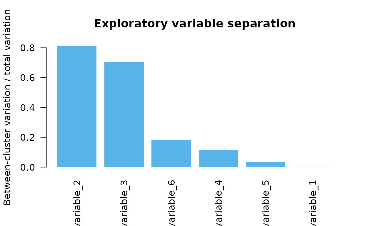
One simple score is the fraction of total variation explained by the posterior modal clusters:

$R_j^2 = \frac{\sum_k n_k(\bar{x}_{jk} - \bar{x}_{j\cdot})^2} {\sum_i (x_{ji} - \bar{x}_{j\cdot})^2}.$

This quantity is not a posterior inclusion probability; it summarizes separation under the fitted partition.

cluster_separation <- function(X, allocation) {
  vapply(seq_len(nrow(X)), function(j) {
    x <- X[j, ]
    overall <- mean(x)
    total <- sum((x - overall)^2)
    between <- sum(vapply(split(x, allocation), function(group) {
      length(group) * (mean(group) - overall)^2
    }, numeric(1)))
    if (total == 0) 0 else between / total
  }, numeric(1))
}

separation <- cluster_separation(X, fit_summary$allocation)
separation_table <- data.frame(
  variable = rownames(X),
  separation = round(separation, 3)
)
separation_table[order(separation_table$separation, decreasing = TRUE), ]
#>     variable separation
#> 2 variable_2      0.810
#> 3 variable_3      0.704
#> 6 variable_6      0.182
#> 4 variable_4      0.114
#> 5 variable_5      0.036
#> 1 variable_1      0.002

ordered <- order(separation, decreasing = TRUE)
barplot(
  separation[ordered],
  names.arg = rownames(X)[ordered],
  las = 2,
  col = "#56B4E9",
  border = NA,
  ylab = "Between-cluster variation / total variation",
  main = "Exploratory variable separation"
)

Bar plot of exploratory variable separation scores.

Compare with loading magnitudes

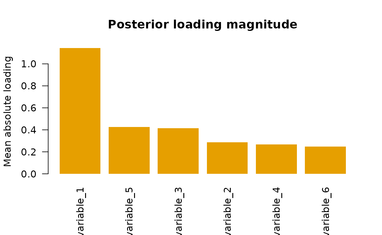
The loading matrices describe how observed variables relate to latent factors inside each component. A simple posterior diagnostic is the average absolute loading magnitude across saved samples and active components.

$L_j = \frac{1}{|\mathcal{S}|} \sum_{s \in \mathcal{S}} \frac{1}{|A_s|} \sum_{k \in A_s} \frac{1}{q_k}\sum_{\ell = 1}^{q_k} |\lambda_{jk\ell}^{(s)}|,$

where $A_s$ is the set of active clusters in posterior sample $s$ . Large $L_j$ means variable $j$ contributes strongly to the latent-factor covariance structure; it is not a posterior inclusion probability.

loading_importance <- function(fit) {
  totals <- NULL
  count <- 0

  for (sample_id in seq_along(fit$lambda_samples)) {
    lambdas <- fit$lambda_samples[[sample_id]]
    active <- which(fit$active_cluster_samples[[sample_id]] == 1)

    for (k in active) {
      lambda <- lambdas[[k]]
      if (!is.matrix(lambda)) {
        next
      }
      score <- rowMeans(abs(lambda))
      if (is.null(totals)) {
        totals <- numeric(length(score))
      }
      totals <- totals + score
      count <- count + 1
    }
  }

  if (count == 0) {
    return(rep(NA_real_, nrow(X)))
  }
  totals / count
}

loading_score <- loading_importance(fit)
loading_table <- data.frame(
  variable = rownames(X),
  mean_abs_loading = round(loading_score, 3)
)
loading_table[order(loading_table$mean_abs_loading, decreasing = TRUE), ]
#>     variable mean_abs_loading
#> 1 variable_1            1.143
#> 5 variable_5            0.425
#> 3 variable_3            0.415
#> 2 variable_2            0.287
#> 4 variable_4            0.267
#> 6 variable_6            0.247

ordered_loading <- order(loading_score, decreasing = TRUE)
barplot(
  loading_score[ordered_loading],
  names.arg = rownames(X)[ordered_loading],
  las = 2,
  col = "#E69F00",
  border = NA,
  ylab = "Mean absolute loading",
  main = "Posterior loading magnitude"
)

Bar plot of average posterior absolute loading magnitudes by variable.

Interpretation

Use both summaries together:

high separation means a variable distinguishes the posterior clusters;
high loading magnitude means a variable contributes to latent-factor covariance structure inside components;
disagreement between the two summaries indicates that the mean structure and covariance structure carry different information.

For formal variable selection, the model would need an explicit variable inclusion prior and posterior inclusion summaries. The current package is best described as supporting model-based clustering, cluster-number selection, and PGMM covariance-structure selection, with exploratory variable prioritization available from posterior outputs.

Suggested reporting language

When using these summaries in a manuscript or analysis report, use wording such as:

We ranked variables by their separation across posterior modal clusters and by posterior loading magnitudes. These rankings are exploratory diagnostics derived from the fitted clustering model, not posterior inclusion probabilities.

Avoid wording such as “selected variables” unless a formal variable-selection model has been fitted. This distinction keeps the statistical target clear and avoids overstating the model.