Getting started with bpgmm

bpgmm fits Bayesian parsimonious Gaussian mixture models for model-based clustering. It targets three posterior inference goals described by Lu, Li, and Love (2021): the partition of observations, the number of clusters, and the cluster covariance structure.

The vignettes have separate roles:

Article	Use it for
data-preparation	matrix orientation, scaling, and choosing m_range and q_new
model-and-sampler	formulas from the paper and their package arguments
examples	inspecting one fitted object
model-selection	RJMCMC summaries for $m$ and covariance model $v$
variable-prioritization	exploratory variable rankings from posterior output
posterior-diagnostics	independent chains, traces, and co-clustering

Fit a model

Input data should be a numeric matrix with variables in rows and observations in columns. The small example below has two variables and eight observations. The example is short so the vignette runs quickly; applied analyses should use larger burn and niter values.

library(bpgmm)
#> bpgmm 1.3.1 loaded. If you use bpgmm in published work, please cite it with citation("bpgmm").

set.seed(2026)

X <- cbind(
  matrix(rnorm(8, mean = -2, sd = 0.2), nrow = 2),
  matrix(rnorm(8, mean = 2, sd = 0.2), nrow = 2)
)
known_labels <- rep(1:2, each = 4)

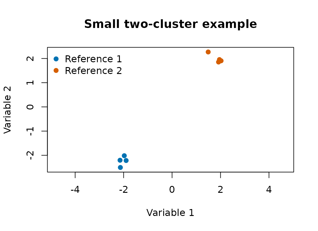
The scatter plot gives a direct check of the simulated partition. Each point is one observation, and the colors show the reference labels used later for the ARI calculation.

plot(
  X[1, ], X[2, ],
  col = c("#0072B2", "#D55E00")[known_labels],
  pch = 19,
  xlab = "Variable 1",
  ylab = "Variable 2",
  main = "Small two-cluster example",
  asp = 1
)
legend(
  "topleft",
  legend = paste("Reference", sort(unique(known_labels))),
  col = c("#0072B2", "#D55E00"),
  pch = 19,
  bty = "n"
)

fit_log <- capture.output({
  fit <- pgmm_rjmcmc(
    X = X,
    m_init = 2,
    m_range = c(1, 3),
    q_new = 1,
    burn = 1,
    niter = 3,
    constraint = model_to_constraint("UUU"),
    m_step = 0,
    v_step = 0,
    verbose = FALSE
  )
})
tail(fit_log, 1)
#> character(0)

The call fixes $m = 2$ and the covariance model so the example is fast. The important arguments are:

• m_init is the initial number of clusters.
• m_range is the allowed range for the number of clusters.
• q_new is the number of latent factors for a new cluster.
• constraint selects the starting covariance model.
• m_step = 1 allows RJMCMC updates for the number of clusters.
• v_step = 1 allows RJMCMC updates across covariance-constraint models.

Summarize posterior samples

summary <- summarize_pgmm_rjmcmc(fit, true_cluster = known_labels)

summary$allocation
#> [1] 2 2 2 2 1 1 1 1
summary$n_clusters
#> 
#> 2 
#> 3
summary$n_constraints
#> 
#> UUU 
#>   3
summary$ari
#> [1] 1

If a reference partition is available, pass it as true_cluster to calculate the adjusted Rand index.

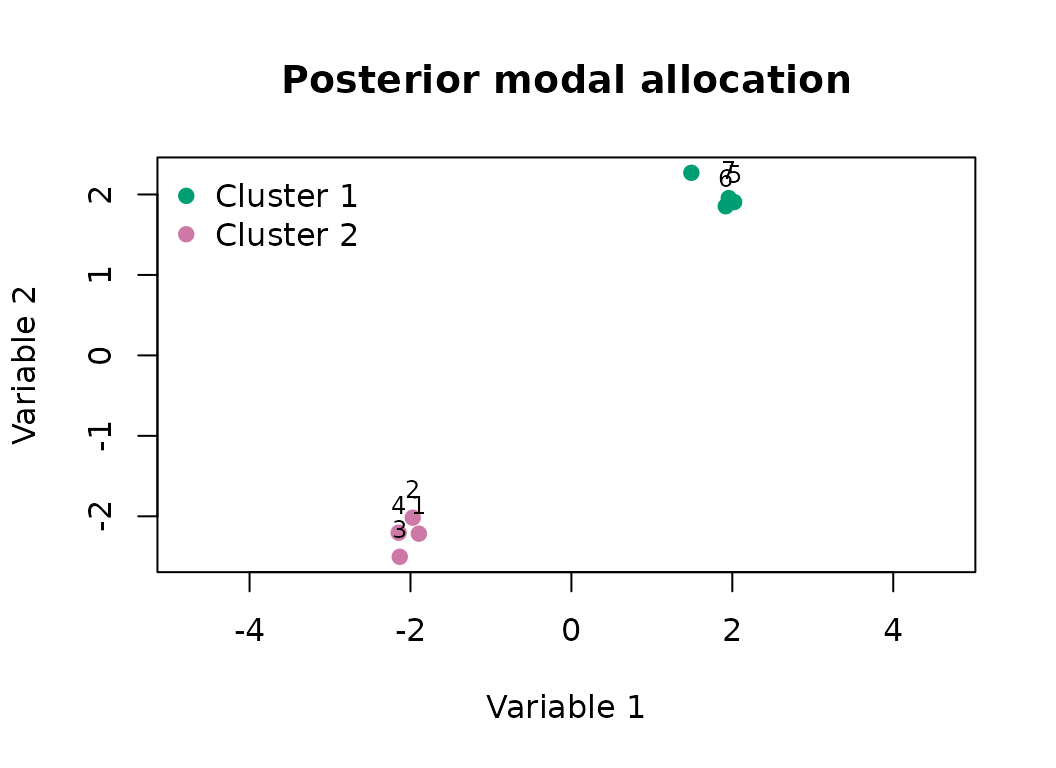
The summary allocation can be plotted back on the original coordinates. This plot is a first check before longer chains and convergence diagnostics.

plot(
  X[1, ], X[2, ],
  col = c("#009E73", "#CC79A7", "#E69F00")[summary$allocation],
  pch = 19,
  xlab = "Variable 1",
  ylab = "Variable 2",
  main = "Posterior modal allocation",
  asp = 1
)
text(X[1, ], X[2, ], labels = seq_along(summary$allocation), pos = 3, cex = 0.75)
legend(
  "topleft",
  legend = paste("Cluster", sort(unique(summary$allocation))),
  col = c("#009E73", "#CC79A7", "#E69F00")[sort(unique(summary$allocation))],
  pch = 19,
  bty = "n"
)

Common early mistakes

Common early problems are:

• X is accidentally supplied as observations by variables instead of variables by observations;
• variables with very different measurement scales are not standardized;
• m_init is outside m_range;
• q_new is too large for a small number of variables;
• m_step and v_step are left at zero when model selection is desired.

Naming convention

Starting with version 1.2.0, the public API uses snake_case names throughout. Use pgmm_rjmcmc(), summarize_pgmm_rjmcmc(), and snake_case argument names such as m_init, m_range, and q_new.

Citation

If you use bpgmm in published work, please cite the package and the methodology paper:

citation("bpgmm")
#> To cite package 'bpgmm' in publications use:
#> 
#>   Lu X, Li Y, Love T (2021). On Bayesian Analysis of
#>   Parsimonious Gaussian Mixture Models. Journal of
#>   Classification, 38, 576-593. doi:10.1007/s00357-021-09391-8
#> 
#> A BibTeX entry for LaTeX users is
#> 
#>   @Article{,
#>     title = {On Bayesian Analysis of Parsimonious Gaussian Mixture Models},
#>     author = {Xiang Lu and Yaoxiang Li and Tanzy Love},
#>     journal = {Journal of Classification},
#>     year = {2021},
#>     volume = {38},
#>     pages = {576--593},
#>     doi = {10.1007/s00357-021-09391-8},
#>   }

Lu, X., Li, Y., & Love, T. (2021). On Bayesian Analysis of Parsimonious Gaussian Mixture Models. Journal of Classification, 38, 576-593. https://doi.org/10.1007/s00357-021-09391-8