Model and sampler details • bpgmm

This section connects the notation in Lu, Li, and Love (2021) to the bpgmm interface. It describes the fitted model, the covariance labels, and the RJMCMC switches used by the sampler. Full fitted examples are given in the getting-started and worked-example vignettes.

Observation model

Let $X = (x_1, \ldots, x_n)$ be a matrix of continuous observations with $p$ variables and $n$ observations. bpgmm expects this same orientation: variables in rows and observations in columns.

For cluster $k$ , the mixture of factor analyzers model writes

$x_i = \mu_k + \Lambda_k y_{ki} + \epsilon_{ki},$

where

$y_{ki} \sim N(0, I_{q_k}), \qquad \epsilon_{ki} \sim N(0, \Psi_k).$

After integrating out the latent factor $y_{ki}$ , the cluster-specific covariance is

$\Sigma_k = \Lambda_k \Lambda_k^\top + \Psi_k.$

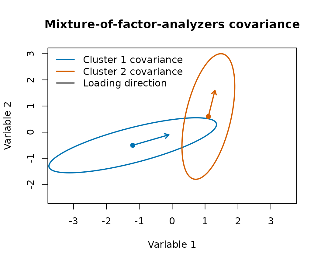
The plot below shows the geometric role of this covariance. The loading matrix $\Lambda_k$ controls the dominant low-dimensional direction, while $\Psi_k$ adds cluster-specific noise around that subspace.

ellipse_points <- function(center, sigma, level = 0.90, n = 120) {
  eig <- eigen(sigma, symmetric = TRUE)
  angles <- seq(0, 2 * pi, length.out = n)
  circle <- rbind(cos(angles), sin(angles))
  radius <- sqrt(qchisq(level, df = 2))
  points <- t(center + radius * eig$vectors %*% diag(sqrt(eig$values), 2) %*% circle)
  colnames(points) <- c("x", "y")
  points
}

lambda_1 <- matrix(c(1.1, 0.4), ncol = 1)
lambda_2 <- matrix(c(0.2, 1.0), ncol = 1)
psi_1 <- diag(c(0.20, 0.08))
psi_2 <- diag(c(0.10, 0.25))
sigma_1 <- lambda_1 %*% t(lambda_1) + psi_1
sigma_2 <- lambda_2 %*% t(lambda_2) + psi_2

ell_1 <- ellipse_points(c(-1.2, -0.5), sigma_1)
ell_2 <- ellipse_points(c(1.1, 0.6), sigma_2)

plot(
  ell_1,
  type = "l",
  lwd = 2,
  col = "#0072B2",
  xlim = c(-3.5, 3.5),
  ylim = c(-2.5, 3),
  xlab = "Variable 1",
  ylab = "Variable 2",
  main = "Mixture-of-factor-analyzers covariance"
)
lines(ell_2, lwd = 2, col = "#D55E00")
points(rbind(c(-1.2, -0.5), c(1.1, 0.6)), pch = 19, col = c("#0072B2", "#D55E00"))
arrows(-1.2, -0.5, -1.2 + lambda_1[1], -0.5 + lambda_1[2], col = "#0072B2", lwd = 2, length = 0.08)
arrows(1.1, 0.6, 1.1 + lambda_2[1], 0.6 + lambda_2[2], col = "#D55E00", lwd = 2, length = 0.08)
legend(
  "topleft",
  legend = c("Cluster 1 covariance", "Cluster 2 covariance", "Loading direction"),
  col = c("#0072B2", "#D55E00", "gray30"),
  lwd = c(2, 2, 2),
  bty = "n"
)

Two covariance ellipses illustrating cluster-specific covariance matrices.

The mixture density is

$f(x_i) = \sum_{k = 1}^m \tau_k N(x_i \mid \mu_k, \Lambda_k \Lambda_k^\top + \Psi_k),$

where $\tau_k$ is the mixture weight and $m$ is the number of clusters. Equivalently, with allocation indicator $z_i \in \{1,\ldots,m\}$ ,

$x_i \mid z_i = k, \Theta \sim N_p(\mu_k, \Sigma_k), \qquad \Pr(z_i = k \mid \tau) = \tau_k .$

In pgmm_rjmcmc():

X is the $p \times n$ data matrix.
m_init is the starting value of $m$ .
m_range is the allowed range of $m$ .
q_new is the factor dimension assigned to a newly proposed cluster.
constraint is the starting covariance model.

PGMM covariance constraints

The paper uses three letters to describe the covariance structure. Each letter is either C for constrained or U for unconstrained.

Letter	Meaning when `C`	Meaning when `U`
1	all clusters share one loading matrix $\Lambda$	each cluster has $\Lambda_k$
2	all clusters share one noise covariance $\Psi$	each cluster has $\Psi_k$
3	noise covariance is isotropic, $\Psi_k = \psi_k I_p$	noise covariance is diagonal

The eight PGMM models are:

library(bpgmm)
#> bpgmm 1.3.1 loaded. If you use bpgmm in published work, please cite it with citation("bpgmm").

models <- c("CCC", "CCU", "CUC", "CUU", "UCC", "UCU", "UUC", "UUU")
data.frame(
  model = models,
  constraint = vapply(
    models,
    function(x) paste(model_to_constraint(x), collapse = ","),
    character(1)
  )
)
#>     model constraint
#> CCC   CCC      1,1,1
#> CCU   CCU      1,1,0
#> CUC   CUC      1,0,1
#> CUU   CUU      1,0,0
#> UCC   UCC      0,1,1
#> UCU   UCU      0,1,0
#> UUC   UUC      0,0,1
#> UUU   UUU      0,0,0

The package uses the numeric encoding internally: 1 means constrained and 0 means unconstrained.

model_to_constraint("UUU")
#> [1] 0 0 0
constraint_to_model(c(1, 1, 0))
#> [1] "CCU"

Priors and posterior updates

The supplement gives the natural conjugate priors used by the MCMC updates. The main priors are:

$\tau \sim \mathrm{Dirichlet}(\gamma, \ldots, \gamma),$

$y_{ki} \sim N(0, I_{q_k}),$

$\mu_k \sim N(\bar{x}, \alpha_1^{-1} \Psi_k),$

$\lambda_{kj} \sim N(0, \alpha_2^{-1} \Psi_k),$

and

$\psi_{kj} \sim \mathrm{IG}(\delta, \beta).$

The complete parameter state can be read as

$\Theta = \{\tau_k, \mu_k, \Lambda_k, \Psi_k, y_{ki}, z_i: k = 1,\ldots,m;\ i = 1,\ldots,n\},$

with hyperparameters

$H = (\alpha_1, \alpha_2, \beta, \delta, \gamma).$

The package samples the hyperparameters $\alpha_1$ , $\alpha_2$ , and $\beta$ , with gamma hyperpriors controlled by:

d_vec: shape parameters.
s_vec: rate parameters.
delta: inverse-gamma shape for the noise covariance.
ggamma: Dirichlet concentration for mixture weights.

The allocation update uses the posterior probability

$p_{ki} = \frac{ \tau_k N(x_i \mid \mu_k, \Psi_k + \Lambda_k\Lambda_k^\top) }{ \sum_{\ell = 1}^{m} \tau_\ell N(x_i \mid \mu_\ell, \Psi_\ell + \Lambda_\ell\Lambda_\ell^\top) }.$

Then

$(z_{i1}, \ldots, z_{im}) \mid X, \Theta, H \sim \mathrm{Multinomial}(1, p_{1i}, \ldots, p_{mi}).$

The allocation update uses this probability, and the joint posterior includes the product of allocated mixture weights:

$p(Z \mid \tau) = \prod_{i = 1}^{n} \tau_{z_i}.$

RJMCMC moves

RJMCMC is used because the number of parameters changes when the number of clusters or the covariance constraint changes.

The cluster-number moves are:

Move	Purpose
stay	update parameters without changing $m$
birth	add a new empty cluster
death	remove an empty cluster
split	split one occupied cluster into two clusters
combine	merge two occupied clusters

The covariance-structure moves toggle one constraint at a time:

toggle whether $\Lambda_k$ is shared across clusters;
toggle whether $\Psi_k$ is shared across clusters;
toggle whether $\Psi_k$ is isotropic or diagonal.

In pgmm_rjmcmc():

m_step = 1 enables birth/death moves for $m$ .
split_combine = 1 adds split/combine moves when m_step = 1.
v_step = 1 enables covariance-constraint moves.

For a proposed move from model $M$ to $M'$ , the RJMCMC acceptance probability has the standard form

$a = \min\left\{ 1, \frac{ p(X, Z, \Theta', H' \mid M')\,p(M')\,q(M \mid M') }{ p(X, Z, \Theta, H \mid M)\,p(M)\,q(M' \mid M) } \left|J\right| \right\},$

where $q(\cdot)$ is the proposal density and $|J|$ is the Jacobian term for dimension-changing moves such as split/combine. Birth/death and split/combine change $m$ ; covariance moves change the constraint label $v \in \{\mathrm{CCC}, \ldots, \mathrm{UUU}\}$ .

Interface mapping

The formula terms map to package output fields as follows:

Paper notation	Package argument or output
$X = (x_1,\ldots,x_n)$	`X`, a $p \times n$ numeric matrix
$m$	`m_init`, `m_range`, `active_cluster_samples`
$q_k$	`q_new` for newly proposed clusters
$z_i$	`allocation_samples`, `summary$allocation`
$\tau_k$	`tau_samples`
$\mu_k$	`mean_samples`
$\Lambda_k$	`lambda_samples`
$\Psi_k$	`psi_samples`
covariance model $v$	`constraint`, `constraint_samples`

An applied model-selection call usually has the following structure:

fit <- pgmm_rjmcmc(
  X = your_data_matrix,
  m_init = 5,
  m_range = c(1, 10),
  q_new = 4,
  burn = 5000,
  niter = 15000,
  constraint = model_to_constraint("UUU"),
  m_step = 1,
  v_step = 1,
  split_combine = 1,
  verbose = FALSE
)

Citation

If you use these methods, cite:

Lu, X., Li, Y., & Love, T. (2021). On Bayesian Analysis of Parsimonious Gaussian Mixture Models. Journal of Classification, 38, 576-593. https://doi.org/10.1007/s00357-021-09391-8

In R:

citation("bpgmm")
#> To cite package 'bpgmm' in publications use:
#> 
#>   Lu X, Li Y, Love T (2021). On Bayesian Analysis of
#>   Parsimonious Gaussian Mixture Models. Journal of
#>   Classification, 38, 576-593. doi:10.1007/s00357-021-09391-8
#> 
#> A BibTeX entry for LaTeX users is
#> 
#>   @Article{,
#>     title = {On Bayesian Analysis of Parsimonious Gaussian Mixture Models},
#>     author = {Xiang Lu and Yaoxiang Li and Tanzy Love},
#>     journal = {Journal of Classification},
#>     year = {2021},
#>     volume = {38},
#>     pages = {576--593},
#>     doi = {10.1007/s00357-021-09391-8},
#>   }