Posterior diagnostics and multiple chains

After fitting bpgmm, posterior samples can be inspected through chain-level summaries, trace plots, and co-clustering probabilities. These diagnostics complement the model-selection example.

The chains below are deliberately short so that the vignette builds quickly. Applied analyses should use longer chains and examine stability across independent runs.

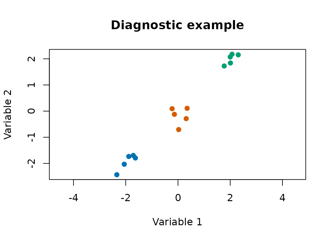
Simulate a diagnostic example

library(bpgmm)
#> bpgmm 1.3.1 loaded. If you use bpgmm in published work, please cite it with citation("bpgmm").

set.seed(2029)
X <- cbind(
  matrix(rnorm(10, mean = -2.0, sd = 0.25), nrow = 2),
  matrix(rnorm(10, mean =  0.0, sd = 0.25), nrow = 2),
  matrix(rnorm(10, mean =  2.0, sd = 0.25), nrow = 2)
)
known_labels <- rep(1:3, each = 5)

cluster_cols <- c("#0072B2", "#D55E00", "#009E73", "#CC79A7")
plot(
  X[1, ], X[2, ],
  col = cluster_cols[known_labels],
  pch = 19,
  xlab = "Variable 1",
  ylab = "Variable 2",
  main = "Diagnostic example",
  asp = 1
)

Run independent chains

pgmm_rjmcmc_chains() runs independent chains. The vignette uses cores = 1 for CRAN portability, but users can increase cores locally.

fits <- pgmm_rjmcmc_chains(
  X = X,
  m_init = 3,
  m_range = c(1, 4),
  q_new = 1,
  burn = 1,
  niter = 4,
  constraint = "UUU",
  m_step = 1,
  v_step = 1,
  chains = 2,
  cores = 1,
  seed = 2029,
  verbose = FALSE
)

length(fits)
#> [1] 2
attr(fits, "chain_seeds")
#> [1] 370199374 178884786

Summarize each chain

For chain $c$, simple empirical summaries are

$$\widehat{p}_c(m = r \mid X) = \frac{1}{S_c}\sum_{s=1}^{S_c} I(m_c^{(s)} = r), \qquad \widehat{p}_c(v = a \mid X) = \frac{1}{S_c}\sum_{s=1}^{S_c} I(v_c^{(s)} = a).$$

Large disagreements across chains are a warning sign, especially when the chains use different random seeds.

chain_summaries <- lapply(fits, summarize_pgmm_rjmcmc, true_cluster = known_labels)

data.frame(
  chain = names(chain_summaries),
  ari = vapply(chain_summaries, function(x) x$ari, numeric(1)),
  modal_clusters = vapply(chain_summaries, function(x) {
    as.integer(names(which.max(x$n_clusters)))
  }, integer(1))
)
#>           chain       ari modal_clusters
#> chain_1 chain_1 1.0000000              3
#> chain_2 chain_2 0.1452145              3

Trace cluster counts and covariance models

The posterior samples store the active cluster indicators and covariance constraint at each saved iteration. These traces are first diagnostics.

cluster_count_trace <- function(fit) {
  vapply(fit$active_cluster_samples, sum, numeric(1))
}

constraint_trace <- function(fit) {
  vapply(fit$constraint_samples, constraint_to_model, character(1))
}

cluster_traces <- lapply(fits, cluster_count_trace)
constraint_traces <- lapply(fits, constraint_trace)

cluster_traces
#> $chain_1
#> [1] 3 3 3 3
#> 
#> $chain_2
#> [1] 3 3 3 3
constraint_traces
#> $chain_1
#> [1] "UUU" "CUU" "CUC" "CCC"
#> 
#> $chain_2
#> [1] "UUU" "UCU" "UCC" "UCC"

old_par <- par(mar = c(4, 4, 3, 1))
plot(
  cluster_traces[[1]],
  type = "b",
  pch = 19,
  ylim = range(unlist(cluster_traces)),
  col = "#0072B2",
  xlab = "Saved iteration",
  ylab = "Active clusters",
  main = "Cluster-count trace"
)
lines(cluster_traces[[2]], type = "b", pch = 19, col = "#D55E00")
legend("topright", legend = names(fits), col = c("#0072B2", "#D55E00"), lty = 1, pch = 19, bty = "n")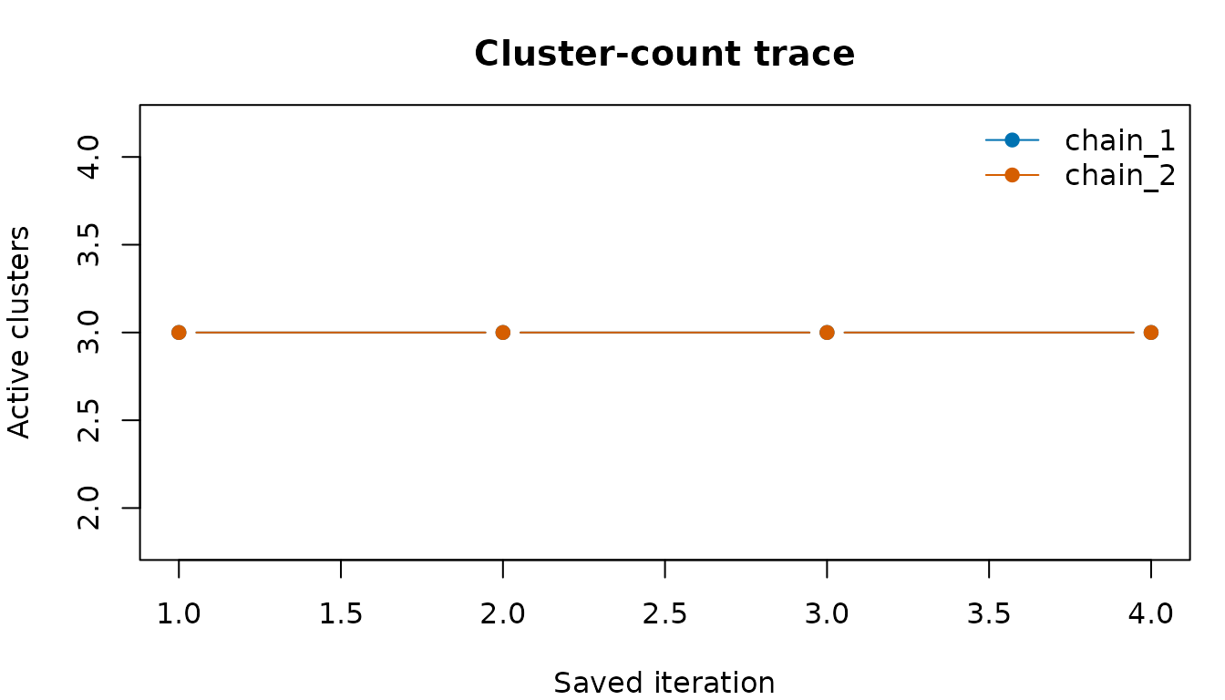

par(old_par)

Posterior co-clustering matrix

A co-clustering matrix estimates how often two observations are assigned to the same cluster across posterior samples. It reports pairwise uncertainty rather than only a single modal allocation.

$$C_{ij} = \Pr(z_i = z_j \mid X) \approx \frac{1}{S}\sum_{s=1}^{S} I\{z_i^{(s)} = z_j^{(s)}\}.$$

co_clustering_matrix <- function(fit) {
  n <- length(fit$allocation_samples[[1]])
  out <- matrix(0, n, n)

  for (allocation in fit$allocation_samples) {
    out <- out + outer(allocation, allocation, "==")
  }

  out / length(fit$allocation_samples)
}

co_mat <- co_clustering_matrix(fits[[1]])
round(co_mat[1:6, 1:6], 2)
#>      [,1] [,2] [,3] [,4] [,5] [,6]
#> [1,] 1.00 1.00 1.00 1.00 1.00 0.25
#> [2,] 1.00 1.00 1.00 1.00 1.00 0.25
#> [3,] 1.00 1.00 1.00 1.00 1.00 0.25
#> [4,] 1.00 1.00 1.00 1.00 1.00 0.25
#> [5,] 1.00 1.00 1.00 1.00 1.00 0.25
#> [6,] 0.25 0.25 0.25 0.25 0.25 1.00

image(
  seq_len(nrow(co_mat)),
  seq_len(ncol(co_mat)),
  co_mat[nrow(co_mat):1, ],
  col = hcl.colors(20, "YlGnBu", rev = TRUE),
  xlab = "Observation",
  ylab = "Observation",
  main = "Posterior co-clustering"
)

What to look for

Warning signs include:

• cluster-count traces that stay at the boundary of m_range;
• very different posterior summaries across independent chains;
• covariance-model traces that never move when v_step = 1;
• co-clustering matrices with no clear block structure;
• sensitivity to scaling, q_new, or m_range.

These diagnostics do not replace a long MCMC analysis, but they give a concise description of the posterior output.