Model selection on a larger simulated MFA data set

The following simulation uses a moderately larger mixture-of-factor-analyzers data set to illustrate model selection in bpgmm. The chain is short so that the vignette builds quickly on CRAN and pkgdown. Applied analyses should use longer burn-in, more posterior samples, multiple chains, and convergence diagnostics.

Simulate clustered factor-analytic data

The simulator below creates three clusters, six observed variables, and two latent factors. The first three variables carry most of the cluster separation, while the last three variables are intentionally less informative.

The generating model matches the paper’s mixture-of-factor-analyzers form:

$$x_i = \mu_{z_i} + \Lambda_{z_i}y_i + \epsilon_i, \qquad y_i \sim N_2(0, I_2), \qquad \epsilon_i \sim N_6(0, \Psi_{z_i}).$$

library(bpgmm)
#> bpgmm 1.3.1 loaded. If you use bpgmm in published work, please cite it with citation("bpgmm").

simulate_mfa_data <- function(n_per_cluster = 20, p = 6, q = 2) {
  means <- rbind(
    c(-3.0, -2.0,  0.0, 0, 0, 0),
    c( 2.5, -1.0,  2.0, 0, 0, 0),
    c( 0.0,  2.5, -2.0, 0, 0, 0)
  )

  lambdas <- list(
    matrix(c(1.2,  0.5, 0.2, 0, 0, 0,
             0.0,  0.2, 0.8, 0.3, 0, 0), nrow = p),
    matrix(c(0.2,  1.1, 0.6, 0, 0, 0,
             0.8,  0.1, 0.2, 0.6, 0, 0), nrow = p),
    matrix(c(0.7, -0.4, 1.0, 0, 0, 0,
            -0.2,  0.8, 0.4, 0.3, 0, 0), nrow = p)
  )

  psi <- list(
    diag(c(0.25, 0.35, 0.30, 0.80, 0.90, 1.00)),
    diag(c(0.30, 0.25, 0.40, 0.80, 0.90, 1.00)),
    diag(c(0.35, 0.30, 0.25, 0.80, 0.90, 1.00))
  )

  n <- n_per_cluster * 3
  X <- matrix(NA_real_, nrow = p, ncol = n)
  true_cluster <- rep(seq_len(3), each = n_per_cluster)

  column <- 1
  for (k in seq_len(3)) {
    for (i in seq_len(n_per_cluster)) {
      latent_score <- rnorm(q)
      noise <- MASS::mvrnorm(1, mu = rep(0, p), Sigma = psi[[k]])
      X[, column] <- means[k, ] + lambdas[[k]] %*% latent_score + noise
      column <- column + 1
    }
  }

  rownames(X) <- paste0("variable_", seq_len(p))
  list(X = X, true_cluster = true_cluster)
}

set.seed(2027)
sim <- simulate_mfa_data()
X <- sim$X
true_cluster <- sim$true_cluster

dim(X)
#> [1]  6 60
table(true_cluster)
#> true_cluster
#>  1  2  3 
#> 20 20 20

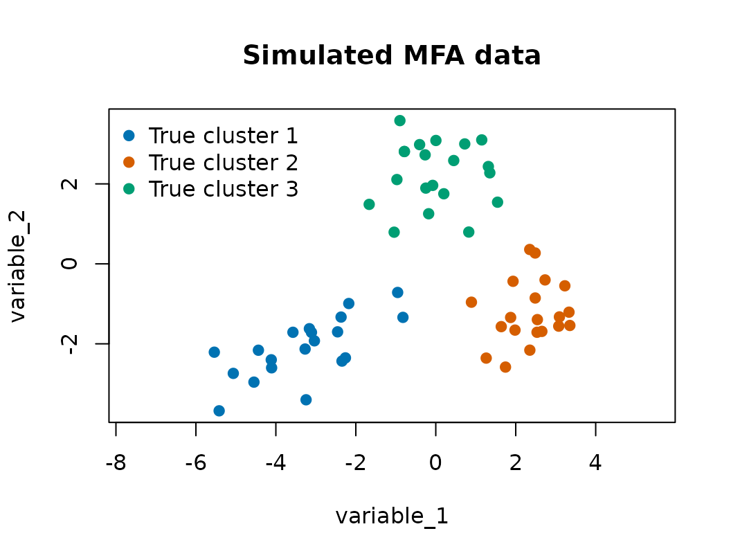
The first two variables already show substantial separation, but the model is fit to all six variables.

cluster_cols <- c("#0072B2", "#D55E00", "#009E73", "#CC79A7", "#E69F00")
plot(
  X[1, ], X[2, ],
  col = cluster_cols[true_cluster],
  pch = 19,
  xlab = rownames(X)[1],
  ylab = rownames(X)[2],
  main = "Simulated MFA data",
  asp = 1
)
legend(
  "topleft",
  legend = paste("True cluster", sort(unique(true_cluster))),
  col = cluster_cols[sort(unique(true_cluster))],
  pch = 19,
  bty = "n"
)

Run RJMCMC model selection

Here m_step = 1 allows the sampler to move across different numbers of clusters, and v_step = 1 allows moves across the PGMM covariance structures. The example uses only a few iterations so that the vignette is fast.

The two discrete targets are

$$p(m \mid X) \quad \text{and} \quad p(v \mid X),$$

where $v$ is one of the eight covariance labels $\{\mathrm{CCC}, \ldots, \mathrm{UUU}\}$. The saved samples estimate these posterior probabilities by empirical frequencies:

$$\widehat{p}(m = r \mid X) = \frac{1}{S}\sum_{s=1}^S I(m^{(s)} = r), \qquad \widehat{p}(v = a \mid X) = \frac{1}{S}\sum_{s=1}^S I(v^{(s)} = a).$$

fit_log <- capture.output({
  fit <- pgmm_rjmcmc(
    X = X,
    m_init = 3,
    m_range = c(1, 5),
    q_new = 2,
    burn = 2,
    niter = 6,
    constraint = "UUU",
    m_step = 1,
    v_step = 1,
    split_combine = 0,
    verbose = FALSE
  )
})
tail(fit_log, 1)
#> character(0)

fit_summary <- summarize_pgmm_rjmcmc(fit, true_cluster = true_cluster)

fit_summary$n_clusters
#> 
#> 3 
#> 6
fit_summary$n_constraints
#> 
#> UCC UCU UUU 
#>   1   1   4
fit_summary$ari
#> [1] 0.9495627

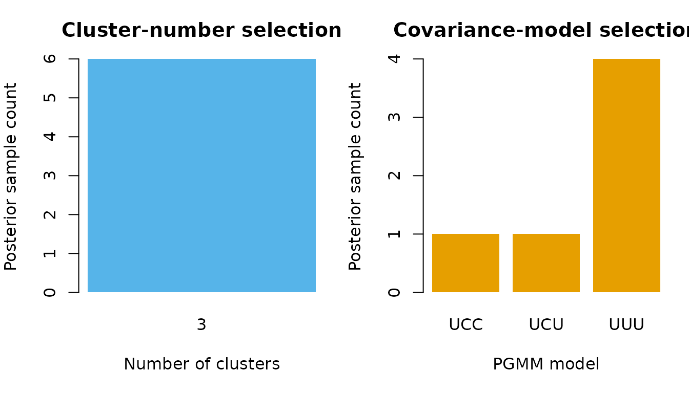
The model-selection summaries are posterior sample counts. In an applied analysis, these bars should be based on a much longer chain.

old_par <- par(mfrow = c(1, 2), mar = c(5, 4, 3, 1))
barplot(
  fit_summary$n_clusters,
  col = "#56B4E9",
  border = NA,
  xlab = "Number of clusters",
  ylab = "Posterior sample count",
  main = "Cluster-number selection"
)
barplot(
  fit_summary$n_constraints,
  col = "#E69F00",
  border = NA,
  xlab = "PGMM model",
  ylab = "Posterior sample count",
  main = "Covariance-model selection"
)

par(old_par)

Compare true and posterior allocations

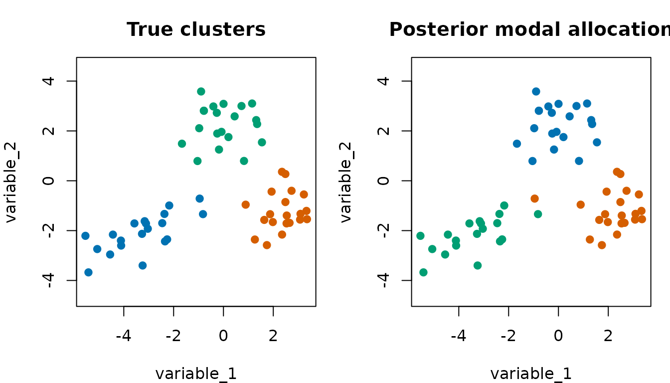
The posterior modal allocation can be plotted against the known simulation labels.

old_par <- par(mfrow = c(1, 2), mar = c(4, 4, 3, 1))
plot(
  X[1, ], X[2, ],
  col = cluster_cols[true_cluster],
  pch = 19,
  xlab = rownames(X)[1],
  ylab = rownames(X)[2],
  main = "True clusters",
  asp = 1
)
plot(
  X[1, ], X[2, ],
  col = cluster_cols[fit_summary$allocation],
  pch = 19,
  xlab = rownames(X)[1],
  ylab = rownames(X)[2],
  main = "Posterior modal allocation",
  asp = 1
)

par(old_par)

Interpreting short versus long runs

The short chain in this vignette demonstrates the mechanics of model selection. It should not be interpreted as a final posterior analysis. In applied work:

• increase burn and niter until summaries are stable;
• compare independent chains with pgmm_rjmcmc_chains();
• check whether sampled cluster counts are stuck at either edge of m_range;
• rerun sensitivity checks for plausible values of q_new;
• inspect whether covariance-model posterior counts change when v_step = 1.

If the posterior mass stays at the upper end of m_range, expand the range or revisit preprocessing. If it stays at the lower end, the data may support fewer clusters than expected, or the covariance model may be too flexible for the sample size.